Chapter 3 - Activation Functions and Derivatives
“Hoping for the best, prepared for the worst, and unsurprised by anything in between.”
— I Know Why the Caged Bird Sings by Maya Angelou
Soon after the invention of the perceptron, people started to create variations of it. A widely used structure is a perceptron that does not have a threshold but instead uses an activation function (we will call this structure a neuron). The key inspiring question or idea that sparked this structure was: how about we keep every component but the threshold, and instead, treat the classification problem as one that is probabilistic? So, there would be a layer of perceptrons in the output layer, but instead of only outputting 0 or 1, all values in between are covered as well. This is essentially the main purpose of the activation function, a function that takes an input and outputs a corresponding value in a given range (usually -1 to 1, or 0 to 1). We will talk about the name’s origin and various widely-used activation functions in this chapter.
In previous chapters, the input of the perceptron was also called the alternative name activation. This seems to coincidentally match the name of this chapter, doesn’t it? Well, it wasn't coincidental when people at the time came up with the names, because activation functions basically adjust the input that goes into a perceptron. To elaborate further, activation functions fit the weighted sum of the inputs and weights of a perceptron and the bias into a range, usually between 0 and 1, but sometimes between -1 and 1 or other ranges, and make the perceptron output this. Since the output of a perceptron is the input of the next layer’s perceptrons, this is where the name activation function comes from. The activation of a perceptron also has another meaning of whether the perceptron fires up(1) or not(0) because neurons in the brain “activate” or light up when the output is 1.
So, what are some commonly used activation functions? Below we will list a few widely used activation functions:
Identity Activation Function
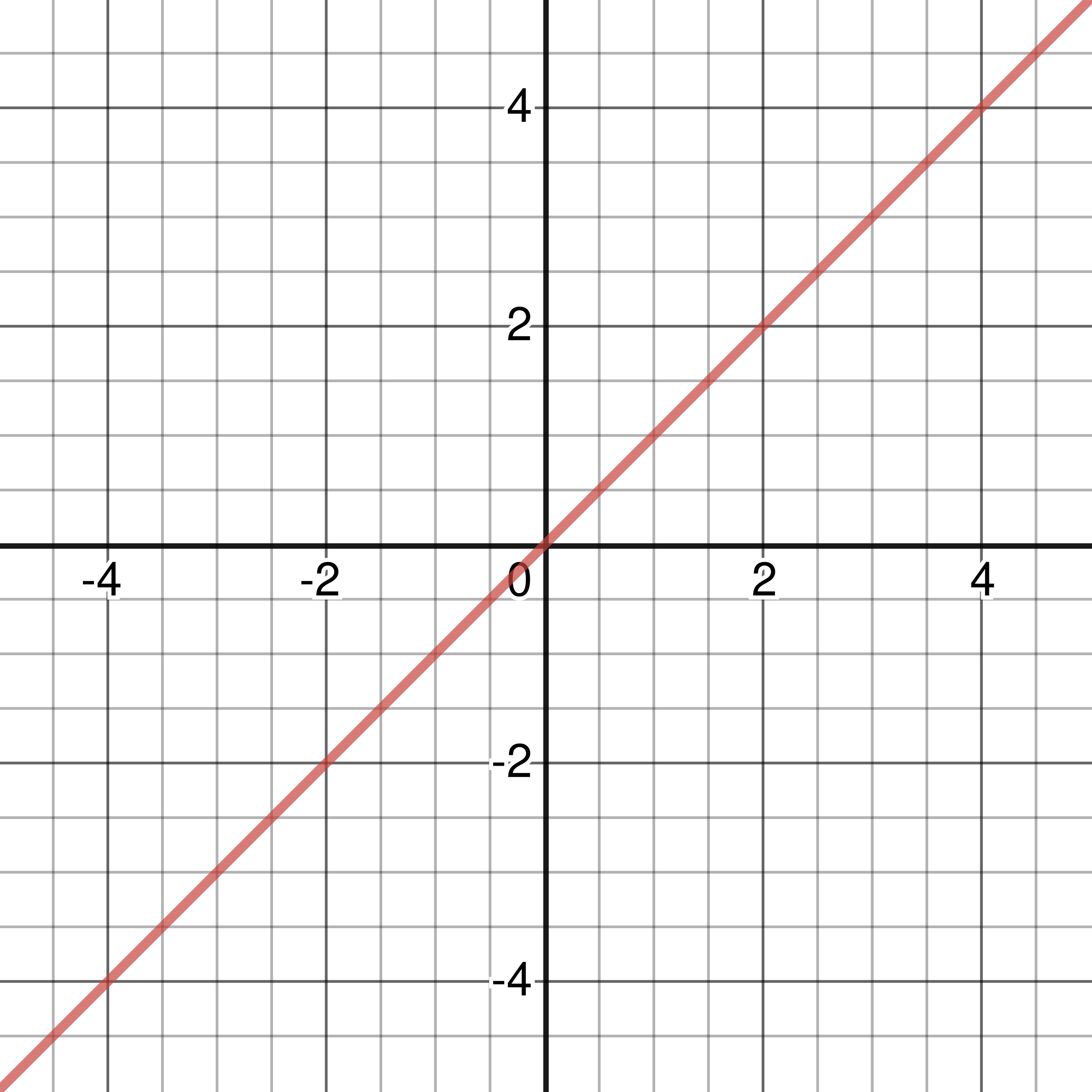
Figure 3-1: Graph of Identity Activation Function
The identity activation function takes the form: \(\sigma(x) = x\), ranging from \(-\infty\) to \(\infty\). The function is linear and its derivative takes the form: \(\sigma\,'(x) = 1\), which makes calculations faster due to its simplicity.
Sigmoid Activation Function
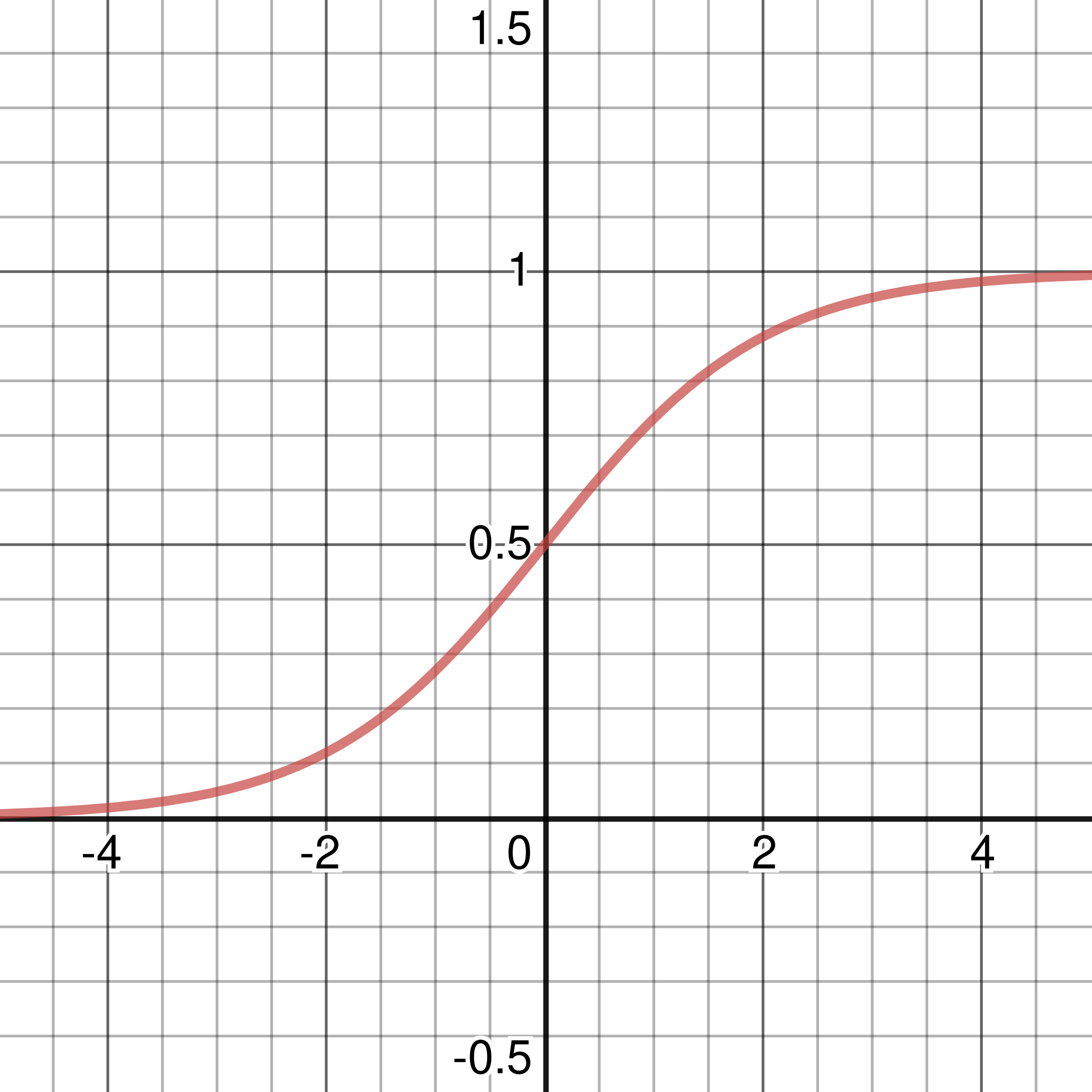
Figure 3-2: Graph of Sigmoid Activation Function
The sigmoid activation function takes the form: \(\displaystyle\sigma(x) = {{1}\over{1\ +\ e^{-x}}}\). The range of the function is between 0 and 1, reaching 0.9 and 0.1 at approximately 2.125 and -2.125 respectively. The sigmoid function is nonlinear and its derivative takes the form: \(\sigma'(x) = \sigma(x)(1 - \sigma(x))\), which is important when using various other learning algorithms that we will talk about like backpropagation. The Sigmoid Function is commonly used to convert a network’s output into a probabilistic output, since its values range from 0 to 1, from uncertain to definite.
TanH Activation Function
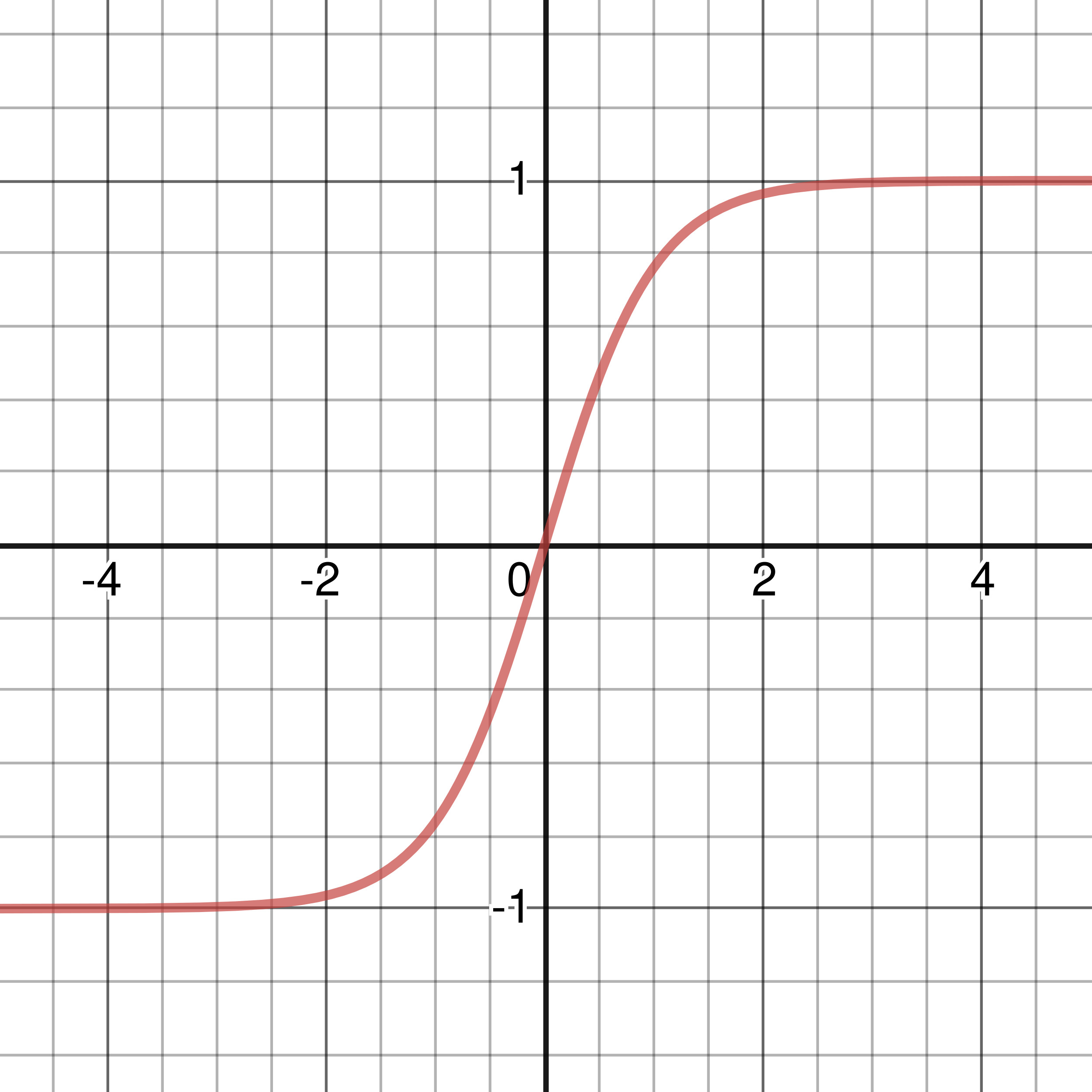
Figure 3-3: Graph of Tanh Activation Function
The tanh activation function takes the form: \(\displaystyle\sigma(x) = {e^{x}\ -\ e^{-x}\over{e^{x}\ +\ e^{-x}}}\). You may notice that it looks quite similar to the sigmoid activation function because it is actually just a squished version of it: another way you can write the tanh activation is: \(\sigma(x) = 2S(2x) - 1\), where \(S(x)\) is the sigmoid function. The derivative of the tanh activation function is: \(\sigma\,'(x) = 1 - \sigma(x)^{2}\). In case you didn’t already know, \(e\) refers to Euler’s number, and is mathematically
expressed as \(\displaystyle\sum^{\infty}_{n\ =\ 0}{1\over{n!}}\), and \(\sigma(x)^{2}\) refers to the square of the result of the tanh activation function.
ReLU Activation Function
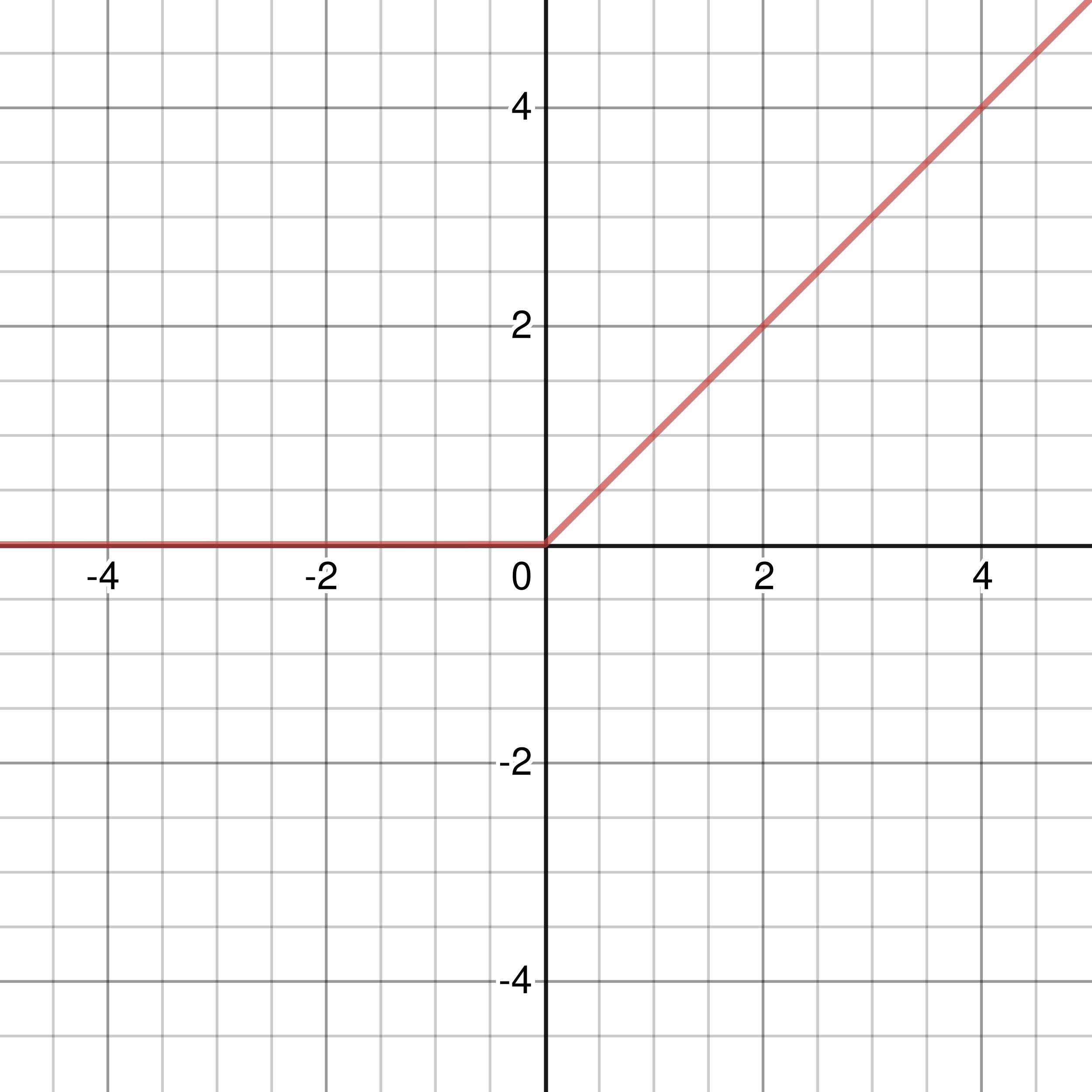
Figure 3-4: Graph of ReLU Activation Function
By far the least computationally expensive, the ReLU activation function takes the form: \(\sigma(x) = \left\{\begin{array}{l} x,\ x > 0 \\ 0,\ x ≤ 0 \end{array} \right.\). What the equation means is, that if the input \(x\) is less than or equal to 0, the function returns 0, otherwise, it returns \(x\) itself. This is arguably the simplest activation function by far and is linear. The derivative for the ReLU activation function is really similar to the function itself: \(\left\{\begin{array}{l} 1,\ x > 0 \\ 0,\ x ≤ 0 \end{array} \right.\)(the only difference is in \(1,\ x > 0\)), and probably is the simplest derivative of all as well.
Leaky ReLU Activation Function
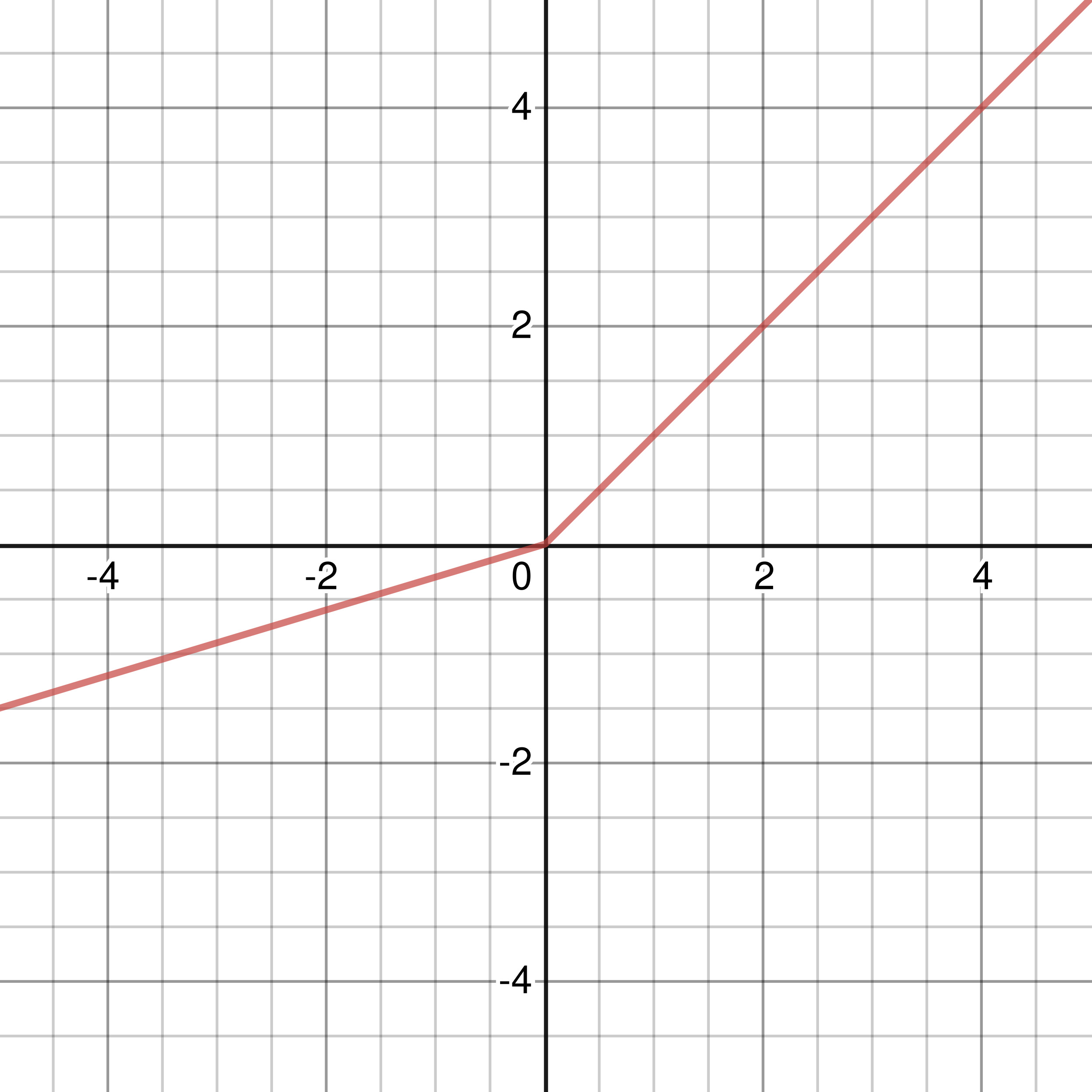
Figure 3-5: Graph of Leaky ReLU Activation Function with \(\left\{\begin{array}{l} x,\ x > 0 \\ 0.3x,\ x ≤ 0 \end{array} \right.\)
Another alternative to the ReLU activation function is the Leaky ReLU. In the graph above, I used \(\left\{\begin{array}{l} x,\ x > 0 \\ 0.3x,\ x ≤ 0 \end{array} \right.\) to better illustrate its difference from the ReLU activation function. Usually, any input less than or equal to 0 is not “leaked” as much as the version I chose above. A popular form of the Leaky ReLU takes the form \(\sigma(x) = \left\{\begin{array}{l} x,\ x > 0 \\ 0.01x,\ x ≤ 0 \end{array} \right.\), and has a derivative of \(\sigma\,'(x) = \left\{\begin{array}{l} 1,\ x > 0 \\ 0.01,\ x ≤ 0 \end{array} \right.\). If you do not know what the derivative of something means, it will be explained later. The complex mathematical symbols will also be explained later in this chapter.
SoftPlus Activation Function
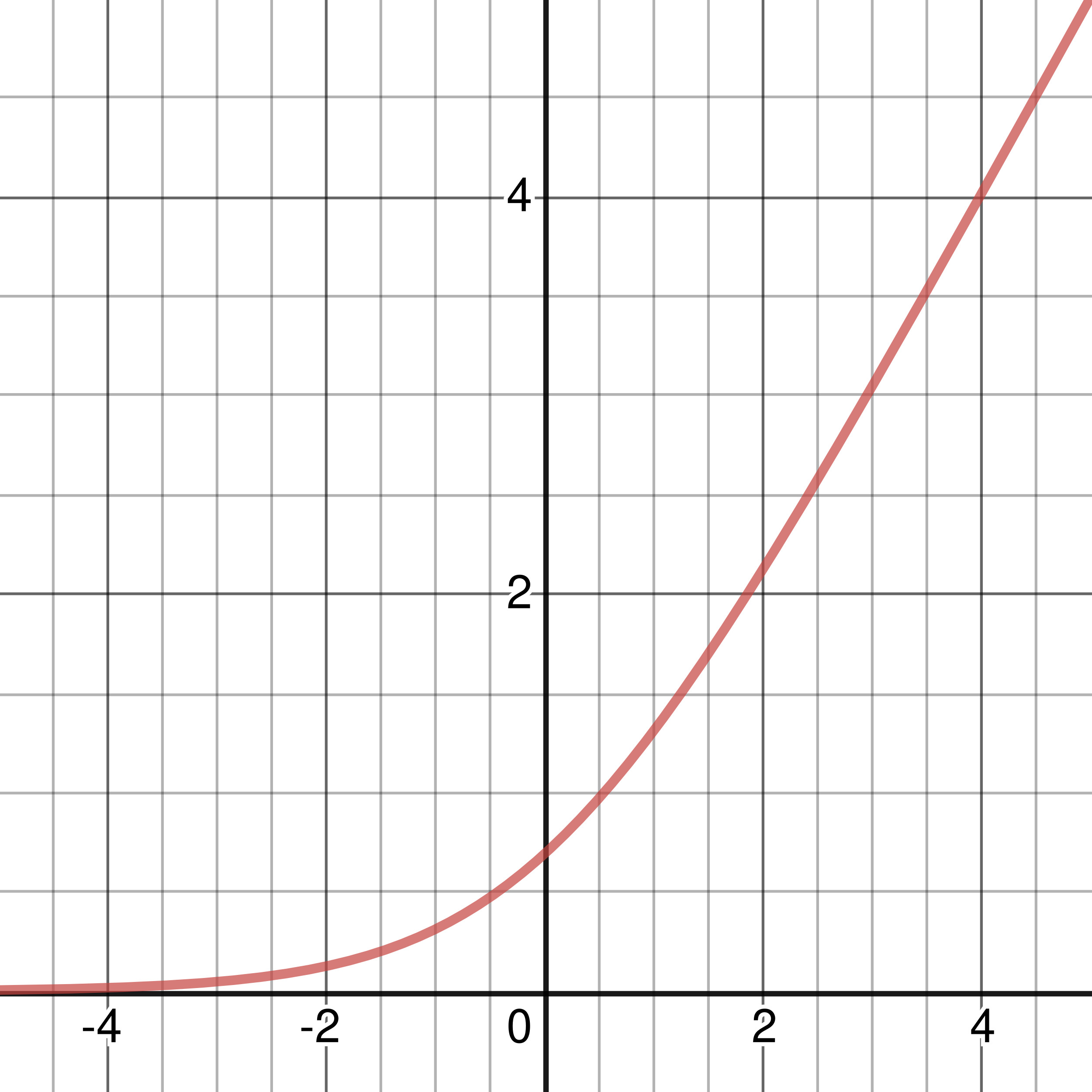
Figure 3-6: Graph of SoftPlus Activation Function
The SoftPlus activation function is another commonly used activation function. Usually, it takes the form: \(\sigma(x) = \ln(1 + e^{x})\) where \(\ln(x)\) refers to the natural logarithm(logarithm base e) of input \(x\). The derivative of the SoftPlus activation function is actually just the sigmoid activation function: \(\displaystyle\sigma\,'(x) = {1\over{1\ +\ e^{-x}}}\). This activation function once again is nonlinear(particularly exponential growth, not linear).
Notation
In my explanations, you may have started noticing an excessive use of the \(\sigma\) (lowercase sigma), to express an activation function. The first activation function that you may have heard of is the sigmoid function, which is named sigmoid because of its S-shaped appearance. Since sigmoid was derived from the character sigma, sigma is used to express the Sigmoid activation function and was conventionally used to express any activation function.
Derivatives
I also talk a lot about derivatives of functions, which is basically a measure of how much a function changes at any given point with respect to any other point on the function, slowly stepping closer and closer to a single point until the distance between the points is 0. In more formal terms, a derivative of a function measures the sensitivity of a given function to change. Basically, how does the tweaking of an input to a function change its output? The process of finding the derivative of a function is called differentiation. The derivative of a function can also be interpreted geometrically as the slope of a line tangent to a single point on the function. Derivatives of an entire function can also be found, where functions’ derivatives are expressed in terms of variables like the ones given above. Another important thing to note about derivatives is that the derivative of a linear function is always equal to the slope of the function. You probably may be thinking: “how do we find a derivative of a single point?” because I haven’t really explained that yet. Well, derivatives first take two points, one being the original point, and the other being one that slowly gets closer and closer to the original point. Call these points \((x, y)\) and \((x+\Delta x, y+\Delta y)\). Then, we keep on decreasing the changes \(\Delta x\) and \(\Delta y\) until the two points are the same, this will therefore give the slope of a function at the single point. By connecting the two points, we are given a line with a slope of \(\displaystyle{\Delta y\over\Delta x}\). \(y\) can also be expressed as \(f(x)\) (function output with input of \(x\)), therefore we can rewrite the points as \((x, f(x))\) and \((x + \Delta x, f(x + \Delta x))\) (note that \(y +\Delta y=f(x+\Delta x)\)). To find the slope, we can use the slope formula (traditionally, rise over run): $$\displaystyle{\Delta y\over{\Delta x}} = {{f(x +\Delta x)-f(x)}\over{x+\Delta x - x}}={{f(x+\Delta x)- f(x)}\over{\Delta x}}$$ Or alternatively: $${{\Delta y}\over{\Delta x}} = {{f(a) - f(b)}\over{a-b}}$$ We use the slope formula because differentiation requires finding the limit of the slope formula, as \(\Delta x\) approaches 0. Expressed mathematically, find: $$\displaystyle\lim_{\Delta x\ \to\ 0}{{f(x\ + \Delta x) - f(x)}\over{\Delta x}}$$ We cannot directly substitute 0 as \(\Delta x\) because this gives: \(\displaystyle{{f(x\ +\ 0)\ -\ f(x)}\over{0}} = {{f(0)}\over{0}}\), which is undefined (divide by 0). Instead, we need to simplify the limit such that substituting \(\Delta x\) with 0 works.
Let’s try an example:
Given \(f(x) = x^{2}\), find \(f'(x)\). Here, \(f'(x)\) represents the derivative of the function and \(f(x)\) represents the function.
This type of notation is usually referred to as Lagrange’s Notation or Prime Notation, because of the use of prime marks(\(\ '\ \)) to represent derivatives.
Other notations commonly used are Leibniz’s Notation, where derivatives are expressed as \(\displaystyle{dy\over{dx}}\) or \(\displaystyle{d\over{dx}}f\); and Newton’s Notation or
Dot Notation, where derivatives are expressed as \(\dot{y}\). Anyway, carrying on, we can substitute the function into limit equation, giving:
\(\displaystyle\lim_{\Delta x\ \to\ 0}{{{x^{2}\ +\ (\Delta x)^{2}\ +\ 2x\Delta x\ -\ x^{2}}\over{\Delta x}}}\)
\(= \displaystyle\lim_{\Delta x\ \to\ 0}{{(\Delta x)^{2}\ +\ 2x\Delta x}\over{\Delta x}}\)
\(= \displaystyle\lim_{\Delta x\ \to\ 0}{\Delta x + 2x}\)
\(= \underline{2x}\)
Therefore, for \(f(x) = x^{2}\), \(f'(x) = 2x\), and \(f''(x) = 2\). \(f''(x)\) means taking the second derivative of the function, or taking the derivative of the derivative of function \(f(x)\). It is not exactly necessary for you to have a very deep understanding of derivatives until we get to the topic of backpropagation, but I have explained it now in case you were curious. If you are a middle school or high school student, you probably won’t have been in contact with derivatives or calculus as a whole, and it is not necessary for you to learn these topics before being taught in school. Instead, just follow my explanations and see if you can understand it. If not, please submit a feedback form or ask/learn about the topics online, on platforms like Khan Academy if you are curious.
It is almost time to start training our own neural network, so head on to the next chapter!
Chapter Summary
- Activation functions replace the threshold of a perceptron, therefore treating classification problems like one that is probabilistic.
- The name activation function is used because activation functions fit all inputs in between a range, which is used as the input or activation of the next layer’s neurons. Also, neurons “activate” or light up(biological neuron) when the output of it is 1.
- Some commonly used activation functions:
- Identity(nothing is changed)
- Function: \(\sigma(x) = x\)
- Derivative: \(\sigma\,'(x) = 1\)
- Sigmoid
- Function: \(\displaystyle\sigma(x) = {{1}\over{1\ +\ e^{-x}}}\)
- Derivative: \(\sigma\,'(x) = \sigma(x)(1 - \sigma(x))\)
- TanH
- Function: \(\displaystyle\sigma(x) = {{e^{x}\ -\ e^{-x}}\over{e^{x}\ +\ e^{-x}}}\), or \(\sigma(x) = 2S(2x) - 1\), where \(S(x)\) is the Sigmoid Activation Function.
- Derivative: \(\sigma\,'(x) = 1 - \sigma(x)^{2}\)
- ReLU
- Function: \(\sigma(x) = \left\{\begin{array}{l} x,\ x > 0 \\ 0,\ x ≤ 0 \end{array} \right.\)
- Derivative: \(\sigma\,'(x) = \left\{\begin{array}{l} 1,\ x > 0 \\ 0,\ x ≤ 0 \end{array} \right.\)
- Leaky ReLU
- Function: \(\sigma(x) = \left\{\begin{array}{l} x,\ x > 0 \\ 0.01x,\ x ≤ 0 \end{array} \right.\)
- Derivative: \(\sigma\,'(x) = \left\{\begin{array}{l} 1,\ x > 0 \\ 0.01,\ x ≤ 0 \end{array} \right.\)
- SoftPlus
- Function: \(\sigma(x) = \ln(1 + e^{x})\) where \(\ln(x)\) refers to the natural logarithm(logarithm base e) of input \(x\).
- Derivative: \(\displaystyle\sigma\,'(x) = {{1}\over{1\ +\ e^{-x}}}\)
- The lowercase sigma is commonly used to symbolise an activation function. It is used because sigmoid was used in the Sigmoid Activation Function’s name because of its S-shape, and because sigmoid came from sigma, and the Sigmoid Activation Function wasn’t the only activation function, and the notation was widely used for it, so all activation functions conventionally were expressed with the lowercase sigma as well.
- Derivatives measure the sensitivity of a function to the change of its input.
- The process of finding derivatives is called differentiation, which is in the field of differential calculus.
- The derivative of a linear function is always equal to its slope.
- Finding the derivative of a single point uses limits, where the distance between two points, one of which was the original, approaches 0.
- The slope formula: \(\displaystyle{{\Delta y}\over{\Delta x}} = {{f(x\ +\ \Delta x)\ -\ f(x)}\over{\Delta x}}\), where \(\Delta x\) and \(\Delta y\) represent the change in \(x\) and \(y\) respectively, given two points \((x,\ y)\) and \((x + \Delta x,\ y + \Delta y)\).
- To find the derivative with the slope formula, simply simplify the limit: \(\displaystyle\lim_{\Delta x\ \to\ 0}{{f(x\ +\ \Delta x)\ -\ f(x)}\over{\Delta x}}\), plugging in the point values or function into the equation.
- Backpropagation requires knowledge on derivatives.